Low Rank Approximation of Kernels
In our paper, titled “Efficient Algorithms for t-distributed Stochastic Neighborhood Embedding”, we present an interpolation scheme for computing the gradient at each iteration of t-SNE. For a numerical analyst, the methods are completely standard, but may be foreign to people without much experience in numerical methods. In this post, I present some background about these numerical methods, with a great emphasis being placed on intuition.
The code in this post is not numerically stable nor optimized; it is only for demonstration purposes. Our actual implementation is available here.
The Problem
Suppose we have $n$ points $\{x_1,…,x_n\}\subset X$ and $m$ points $\{y_1,…,y_m\} \subset Y$, a kernel $K: X \times Y \rightarrow \mathbb R$, and we are interested in computing the following sum, for $i=1,…,n$.
Computed naively, the sums would take $n\cdot m$ time, which is prohibitive for large $n,m$.
Suppose we know that $K$ was low-rank, that is, there are basis functions $u_l:X\rightarrow \mathbb R$ and $v_l: Y \rightarrow \mathbb R$ for $l=1,…,k$ such that
Now, just plugging in:
Note that $m_l$ is only computed once for all $i$, meaning that the sums can be computed in $k(m+n)$ computations–a dramatic improvement over $m\cdot n$!
In other words, supposing we had the $u_l, v_l$, the computation of this sum would be as follows:
Step 1: Compute $m_l = \sum_j v_l(y_j)q(y_j)$ for each $l=1,…,k$
Step 2: Compute $f(x_i) \approx \sum_l u_l(x_i)\sigma_l m_l$ for $ i=1,…,n$
Clearly, it is highly desirable to find functions $u_l,v_l$. When is this possible? And what kind of functions will work?
Optimal Approximation with SVD
Before we answer this, let’s reformulate the above sums in terms of matrix multiplications, by assuming $X,Y \subset \mathbb R$, $q\in \mathbb R^m$, and $K \in \mathbb R^{n\times m}$. The goal is to compute the vector $f \in \mathbb R^n$:
We know from the Eckart-Young-Minsky theorem that the optimal (in terms of L2 and Frobenius norm) approximation to $K$ is the Singular Value Decomposition (SVD):
where $U\in \mathbb R^{m \times k}$ with orthonormal columns $u_1,…,u_k$, $V \in \mathbb R^{n\times K}$ with orthonormal columns $v_1,…,v_k$, and diagonal matrix $\Sigma \in \mathbb R^{K \times K}$ with $\sigma_1,…,\sigma_k$ along the diagonal.
Let’s use the SVD to compute a low-rank approximation to the following two kernels, $K_1$ and $K_2$:
Notice that $K_1$, which is the Cauchy kernel (and the one we deal with in the paper), does not go towards infinity when $x$ approaches $y$. On the other hand, $K_2$ approaches infinity when $x$ approaches $y$, and hence, we will see that for near field interactions, it is not low rank.
Let’s demonstrate in MATLAB by generating random points on the unit interval. Here, $X=Y$, that is, all points interact with all points.
rng(1)
a = 0; b=1; n = 1000;
[locs,~] = sort(rand(n,1)*(b-a));
distmatrix = squareform(pdist(locs));
kernel1 = 1./(1+distmatrix.^2);
kernel2 = 1./(distmatrix.^2);kernel2(kernel2==Inf) = 0;


[U1, S1, V1] = svd(kernel1);
[U2, S2, V2] = svd(kernel2);
figure(1)
semilogy(diag(S1), 'linewidth',4); hold on
semilogy(diag(S2), 'linewidth',4);
legend('K_1', 'K_2'); title('Spectra of Kernels: Neear Field Interactions'); set(gca,'FontSize',12)
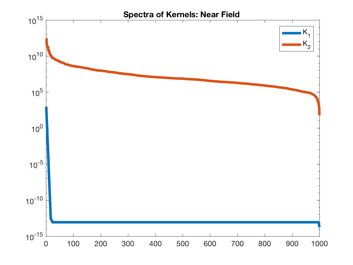
Note how the singular values of $K_1$ decay immediately to zero, whereas $K_2$ decays from $10^{12}$ to $10^9$. This is what we mean by low-rank kernel: the matrix $K$ is a linear combination of very few vectors. Now, let’s compute the relative error as $\| USV^Tq - f\|/\|f\|$ for both of these kernels as a function of $k$.
q = sin(10*locs) + cos(2000*locs); %Anything could be used here

%Exact
f1 = kernel1*q;
f2 = kernel2*q;

ks = [1:20 100 200];
K1_svd_errors = ones(length(ks),1); K2_svd_errors = ones(length(ks),1);
for ki =1:length(ks),
    k = ks(ki);
    kernel1_approx = V1(:,1:k) * S1(1:k,1:k) * V1(:,1:k)';
    f1_approx = kernel1_approx*q;
    K1_svd_errors(ki) = norm(f1_approx - f1)/norm(f1);

    kernel2_approx = V2(:,1:k) * S2(1:k,1:k) * V2(:,1:k)';
    f2_approx = kernel2_approx*q;
    K2_svd_errors(ki) = norm(f2_approx - f2)/norm(f2);
end

figure(2); clf
semilogy(ks,K1_svd_errors,'linewidth',2);
hold on
semilogy(ks,K2_svd_errors,'linewidth',2);
ylabel ('Relative error'); xlabel('k'); set(gca,'FontSize',12); title('Optimal Rank-k Approximation: Near Field');
legend('K_1', 'K_2');
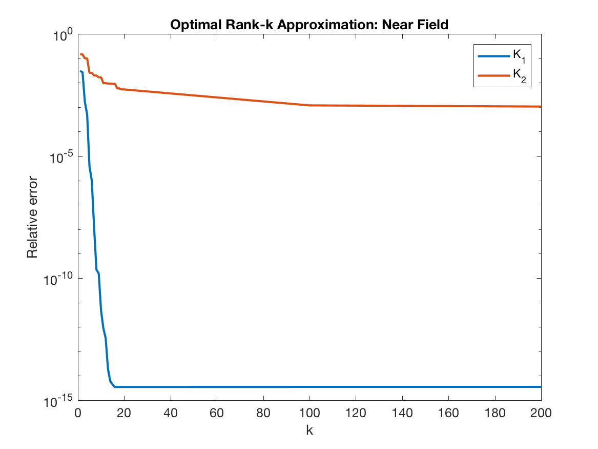
With <20 vectors, we can approximate $K_1$ to machine precision, but not the case for $K_2$, we can only get about 3 digits, which can be seen by taking the log of the condition number as $\log(10^{12}/10^9)$ =3.
The problem with $K_2$ is that it explodes to infinity for points that are too close. Indeed, if the interaction of well-separated points is being calculated, then $K_2$ is also low rank.
a1 = 0; b1=1;
a2 = 2; b2 = 3;
n = 1000;
[locs1,~] = sort((b1+a1)/2+ rand(n,1)*(b1-a1));
[locs2,~] = sort((b2+a2)/2+rand(n,1)*(b2-a2));

distmatrix = squareform(pdist([locs1; locs2]));
kernel1 = 1./(1+distmatrix(1:1000,1001:2000).^2);
kernel2 = 1./(distmatrix(1:1000,1001:2000).^2);kernel2(kernel2==Inf) = 0;

[U1, S1, V1] = svd(kernel1);
[U2, S2, V2] = svd(kernel2);
figure(100)
semilogy(diag(S1), 'linewidth',4); %xlim([0,500]);
 hold on
semilogy(diag(S2), 'linewidth',4);%xlim([0,500]);
legend('K_1', 'K_2'); title('Spectrum of kernels'); set(gca,'FontSize',12)
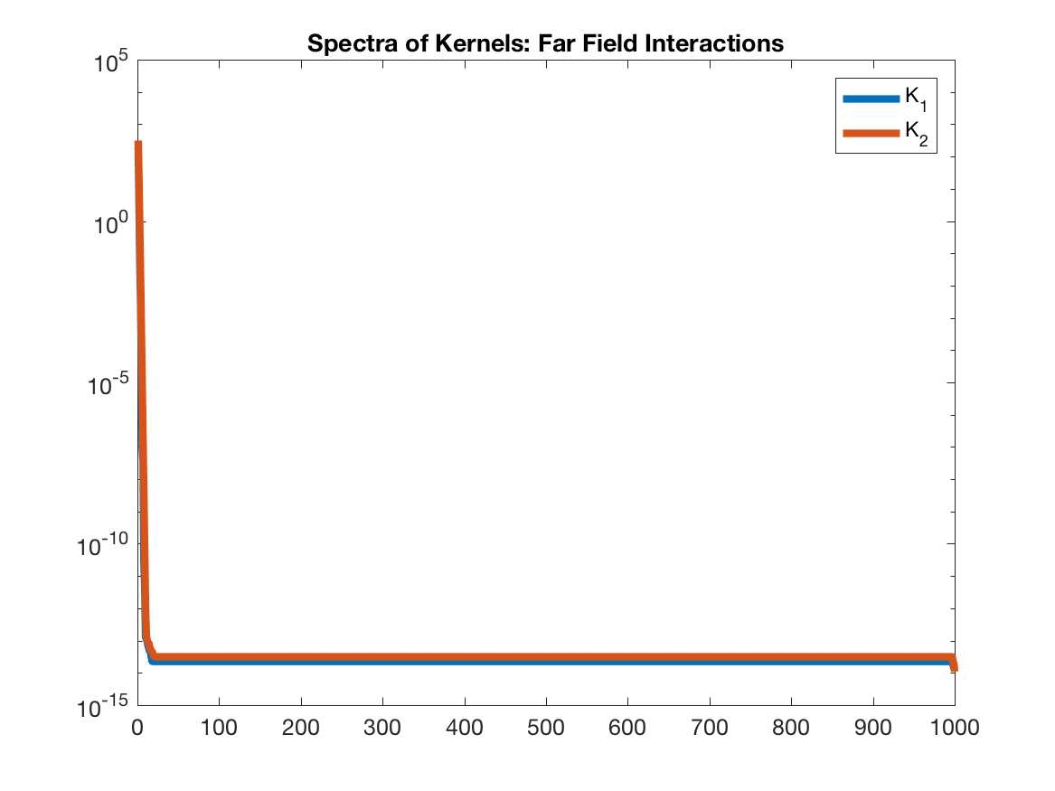
If we were interested in approximating $K_2$, then we could use a fast multipole method (FMM), which treats the interaction between points close to eachother (near field) differently that points far from eachother (far field). In the near field, the interactions are directly computed, whereas in the far field, they are approximated. For example, check out the Black Box FMM of Fong and Darve (paper).
But for t-SNE, we need to approximate $K_1$, which is low rank for all interactions, and hence we don’t need that kind of machinery. We can use the same approximation for all interactions.
Polynomial Interpolation
The SVD gives the optimal low-rank approximation, as it gives a basis for $X$ and $Y$ that is specific to $K$, but it is unfortunately not practical in this setting. Forming the matrix $K$ is itself an $m\cdot n$ operation, which is prohibitive even before we start to compute the SVD.
Instead, we will use polynomial interpolation. Fix $y_0$, and consider $f(x) = K(x,y_0)$, which is only a function of x. Let $\{x_1’,…,x_k’\}$ be points on the interval containing $X$, which we call interpolation points. We will now construct a $k$th-degree polynomial $L(x)$ such that $L(x_i’) = f(x_i’)$ for $i=1,…,k$
which is a linear combination of Lagrange basis polynomials
The trick here is that $u_i(x_j’) = 1$ for $i=j$, but is zero otherwise. Therefore, $L$ will equal $f$ at each of the interpolation points. Similarly, we define interpolation points $\{y_1’,…,y_k’\}$ for $Y$, and Lagrange basis polynomials $v_l(x)$ for $l=1,…,k$. With these basis polynomials, we can compute $f$ as
It can be easily seen that this is also a matrix factorization. Let $u_i=\left[u_i(x_1), u_i(x_2),…,u_i(x_m)\right]^\top$ and $v_i=\left[v_i(x_1), v_i(x_2),…,v_i(x_n)\right]^\top$ for $i=1,…,k$. Concatenate these into an $m \times k$ matrix $U$ and $n \times k$ matrix $V$, respectively. Now define a $k \times k$ matrix $S$, with $S_{i,j} = K(x_i,x_j)$ for $i,j=1,…,k$, and we have
Let’s try it with our kernel $K_1$ from above. Note that this kernel is symmetric, so $u_i = v_i$, and $U=V$.
ps = 1:15;
K1_poly_errors = ones(length(ps),1);

%With varying number of interpolation points
for pi=1:length(ps)
    h = (b-a)/ps(pi); % Distance between interpolation points
    interp_points = a:h:b;
    k = length(interp_points);% Number of interpolation points

    V = zeros(n,k); %Columns of V will form our polynomial basis

    % There are k Lagrange polynomials (one for each point), evaluate each
    % of them at all the n points

    %Note how this is entirely independent of the kernel!
    for ti=1:length(interp_points),
        for yj=1:n
            num = 1;
            denom = 1;
            for tii=1:k
                if (tii ~= ti)
                    denom = denom*(interp_points(ti) -interp_points(tii));
                    num= num*(locs(yj) - interp_points(tii));
                end
            end

            V(yj,ti) = num/denom;
        end
    end

    %We only evaluate the kernel at the k by k interpolation points
    S = ones(k,k);
    for i=1:k
        for j=1:k
            S(i,j) = 1/(1+norm(interp_points(j)-interp_points(i))^2);
        end
    end

    f1_poly_approx = V*S*V'*q;
    K1_poly_errors(pi) = norm(f1_poly_approx - f1)/norm(f1);
end

figure(5); clf
semilogy(ps,K1_poly_errors,'linewidth',2);
hold on
semilogy(ks(1:20),K1_svd_errors(1:20), 'linewidth',2)
ylabel ('Relative error'); xlabel('k'); set(gca,'FontSize',12); title('Polynomial rank-k approximation');
legend('Lagrange Polynomial', 'SVD')
Note that the matrix $V$ is entirely independent of the kernel. As you can see below, the error decreases, but as discussed above, SVD is better.
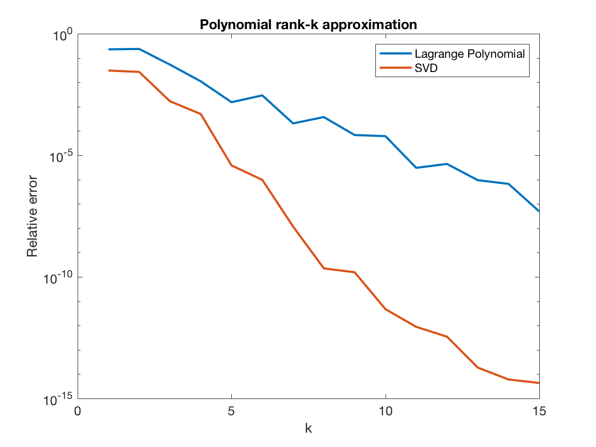
Remarkably, the error is independent of the number of points $n$. And most importantly, it does not require formation of the matrix $K$, so it can be applied to millions of points with very little time and memory.
Note that I formed the matrices V and S because I think the connection with matrix decomposition is very nice, but this is not done in practice as it is terrible numerically. Instead, we just directly compute the sums.
Improving Accuracy with Subintervals
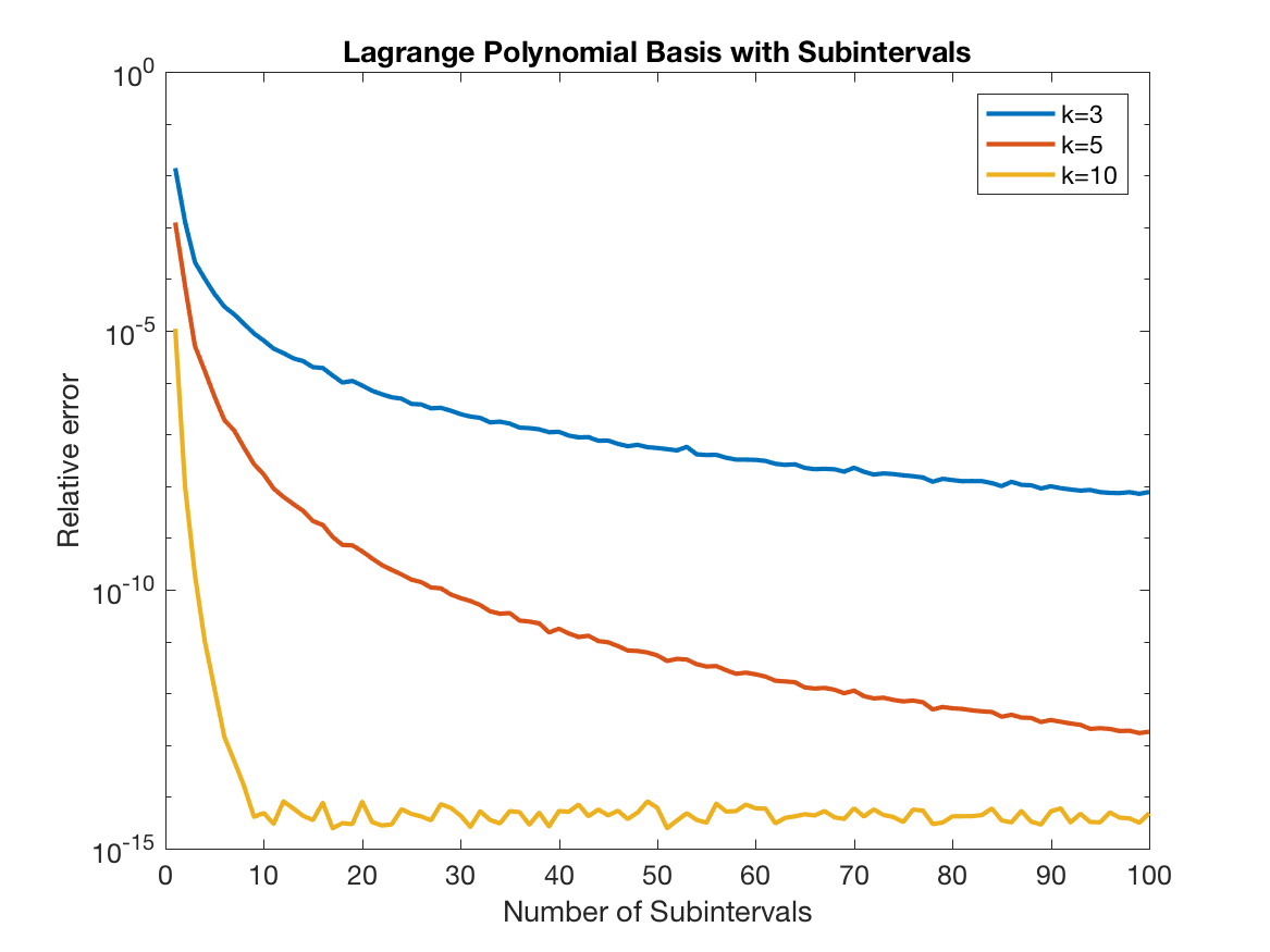
The procedure above is not numerically stable, and given the equispaced interpolation points, it also will suffer from the Runge phenomenon as $k$ increases. So, instead of using $k$ interpolation points for the whole interval, we split the interval into $N_{int}$ sub-intervals, each with $k$ interpolation points. Then, we interpolate each point using the interpolation points within its interval. The key point here is that because we are interpolating on small intervals, we can achieve machine precision, with small $k$.
 To see how this works, let’s
visualize the resulting $V$ and $S$ matrices, with $N_{int}=5$ and $k=3$.
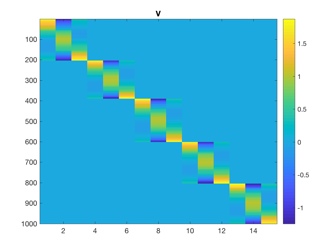
Take a look at the first 200 rows of $V$, and notice how only the first
three columns are nonzero? These are the Lagrange polynomials corresponding to the
$k=3$ interpolation points of the first interval evaluated at the ~200 points
in that interval. In other words, the whole interval is represented by just those three points. And the same for all the other 4 intervals.
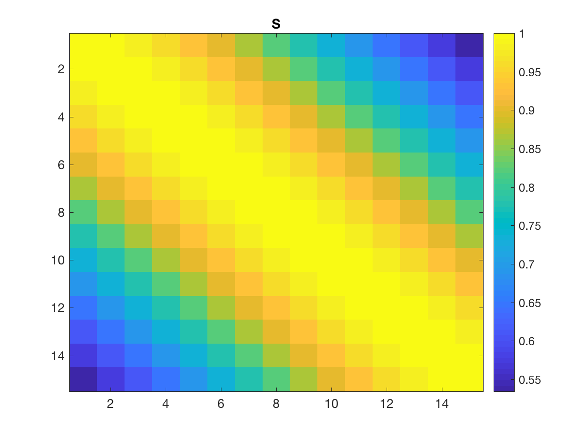
Now, $S$ contains all the interactions between all the nodes (across all intervals), that’s why it is $kN_{int} \times kN_{int}$. So, $V^T$ “sends” the points to the interpolation nodes, $S$ computes their interaction, and $V$ sends them back to the original points!
Take a look at the code:
k = 2;
Nint = 5; %Number of intervals
h = 1/(Nint *k);

%k interpolation points in each interval
interp_points = zeros(k,Nint);
for j=1:k
    for int=1:Nint
        interp_points(j,int) = h/2 + ((j-1)+(int-1)*k)*h;
    end
end

%We need to be able to look up which interval each point belongs to
int_lookup = zeros(n,1);
current_int = 0;
for i=1:n
    if (k*h*(current_int) < locs(i))
        current_int = current_int +1;
    end
   int_lookup(i) = current_int;
end

%Make V, which is now n rows by Nint*k columns
V = zeros(n,Nint*k);
for ti=1:k
    for yj=1:n
        current_int = int_lookup(yj);
        num = 1;
        denom = 1;
        for tii=1:k
            if (tii ~= ti)
                denom = denom*(interp_points(ti,current_int) -interp_points(tii,current_int));
                num= num*(locs(yj) - interp_points(tii,current_int));
            end
        end

        V(yj,(current_int-1)*k+ti) = num/denom;
    end
end

%Make S, which is k*Nint by k*Nint
S = ones(k*Nint,k*Nint);
for int1=1:Nint
    for i=1:k
        for int2=1:Nint
            for j=1:k
                S((int1-1)*k+i,(int2-1)*k+j) = 1/(1+norm(interp_points(i,int1)-interp_points(j,int2))^2);
            end
        end
    end
end

f1_poly_approx = V*S*V'*q;
Extending to Two Dimensions
In two dimensions, everything is analogous; but with tensor products not matrix products. We need to divide each dimension into $N_{int}$ subintervals, resulting in a grid with $(p\cdot N_{int})^2$ points. The problem, however, is that $K$ is now a matrix of size $(p\cdot N_{int})^2 \times (p\cdot N_{int})^2$, which is very large. Because we are using equispaced nodes, and because $K$ can be embedded in a Toeplitz matrix of twice its size, we can use the Fast Fourier Transform to perform the multiplication in the Fourier domain. This is, in fact, the reason why we chose to use equispaced nodes in the first place: it allows us to use the FFT to accelerate the matrix multiplication. Please see the paper for more details.
Final Thoughts
I am indebted to Manas Rachh and Jeremy Hoskins, from whom I learned most of this material.
Please let me know if you find any errors, or have any questions/comments!