Some uses of defects in quantum field theory
Andrew NeitzkeUniversity of Texas at Austin
thanks to many people here for help (all errors and omissions are still mine)


What is quantum field theory?
There's a diversity of views on this question.
Better get an expert's opinion...
An expert opinion
Nathan Seiberg was recently awarded the Fundamental Physics Prize for "major contributions to our understanding of quantum field theory and string theory."
At the 2014 Breakthrough Prize Symposium, he gave a talk entitled "What is quantum field theory?"
The state of play
Quantum field theory has been enormously effective in diverse areas, including:
- particle physics
- condensed matter
- string theory/quantum gravity
- geometry/topology
- algebra/representation theory
Despite this, we do not have a satisfactory definition of QFT, let alone proofs of important "facts" about QFT.
The role of defects
There is a growing sense that one of the reasons why QFT is hard to understand is that we have not fully appreciated the role of defects: lines, surfaces, volumes, $\dots$, inserted in spacetime.

Along a defect, the theory is modified in some way.
Old outlook: defects are optional; have useful applications, but probably are not part of the core of what a QFT is.
New outlook: defects are essential; must be built into the story from the very beginning.
Defects where?
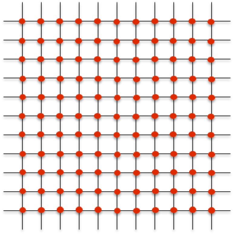
Condensed matter physicists probably do not need convincing that defects are important!
Boundaries and domain walls are well known objects of study. Also lower-dimensional defects e.g. a line of atoms missing from a lattice.

It's perhaps less obvious that defects are also important in particle physics applications of QFT: after all, there is no luminiferous ether...
The plan
First, some specific (old and new) applications of defects in particle physics.
Then, an emerging picture of how defects can help us define QFT.
Local operators
Let's start with zero-dimensional defects, also called local operators.What we learn about QFT in textbooks
A QFT is a machine which produces correlation functions of local operators, inserted at points of spacetime.

$$\langle \phi_1(x_1) \phi_2(x_2) \cdots \phi_n(x_n) \rangle$$
Defining the correlation functions
Textbook recipe for correlation functions uses:
-
Fields on spacetime: e.g. $\phi(x)$, $A_\mu(x)$, $\psi_\alpha(x)$
The fields fluctuate, explore all possible configurations.
- Action: a "weight" for fields $$ S = \int_{{\mathbb R}^d} \partial_\mu \phi \partial^\mu \bar\phi + g^4 \lvert \phi \rvert^4 $$

Then correlation function
$$\langle \phi(x_1) \phi(x_2) \phi(x_3) \rangle$$
is like weighted average of $\phi(x_1) \phi(x_2) \phi(x_3)$ over all possible field configurations.
Correlation functions at work
The Fourier transforms of correlation functions of local operators give scattering amplitudes: main objects of interest for application to particle physics.
The viewpoint that "correlation functions are all QFT is" has been very influential. Indeed there have been many attempts to define a QFT as a collection of correlation functions obeying a list of axioms (e.g. Osterwalder-Schrader 1973).
Line defects
Now let's see a situation where one-dimensional line defects are crucial for understanding the physics: confinement and duality in Yang-Mills theory in four spacetime dimensions.
Yang-Mills theory
Fix a compact Lie group $G$ ("gauge group") with Lie algebra ${\mathfrak g}$.
e.g. $G = SU(N)$, the $N \times N$ unitary matrices of determinant $1$; then ${\mathfrak g} = su(N)$, the $N \times N$ traceless skew-Hermitian matrices.

The Yang-Mills field is $4$ elements $A_\mu(x) \in \mathfrak g$ at each point $x$ of spacetime, where $\mu = 0,1,2,3$ is a vector index.
The Yang-Mills action is $$ S = \frac{1}{g^2} \int d^4x\, {\mathrm{Tr}}\,F_{\mu \nu} F^{\mu \nu} $$ where $$ F_{\mu \nu} = \partial_\mu A_\nu - \partial_\nu A_\mu + [A_\mu, A_\nu] $$
Electromagnetism
When the group $G = U(1)$ (the circle group), Yang-Mills theory reduces to (quantum) electromagnetism. In that case $F_{\mu \nu}$ is the electromagnetic field:
$$ F = \begin{pmatrix} 0 & E_x & E_y & E_z \\ -E_x & 0 & B_z & B_y \\ -E_y & -B_z & 0 & B_x \\ -E_z & -B_y & -B_x & 0 \end{pmatrix} $$$A_\mu$ combines the scalar and vector potentials:
$$ A = \begin{pmatrix} V \\ A_x \\ A_y \\ A_z \end{pmatrix} $$So Yang-Mills theory is like a multi-component, nonlinear version of electromagnetism.
Gauge equivalence
As in electromagnetism, sometimes different Yang-Mills field configurations $A_\mu(x)$, $A'_\mu(x)$ are counted as equivalent: this happens if there exists a gauge transformation $g(x) \in G$ with
$$A'_\mu(x) = g(x)^{-1} A_\mu(x) g(x) + g(x)^{-1} \partial_\mu g(x)$$Electric charges in Yang-Mills theory
In electromagnetism, the electric charge carried by a particle is an integer.

In Yang-Mills theory the nonabelian electric charge carried by a particle lies in some representation of $G$. Each representation can be viewed as a package of weights which label individual particle types.
For example: the strong nuclear force is governed by Yang-Mills theory with $G = SU(3)$. Here are some representations that appear:

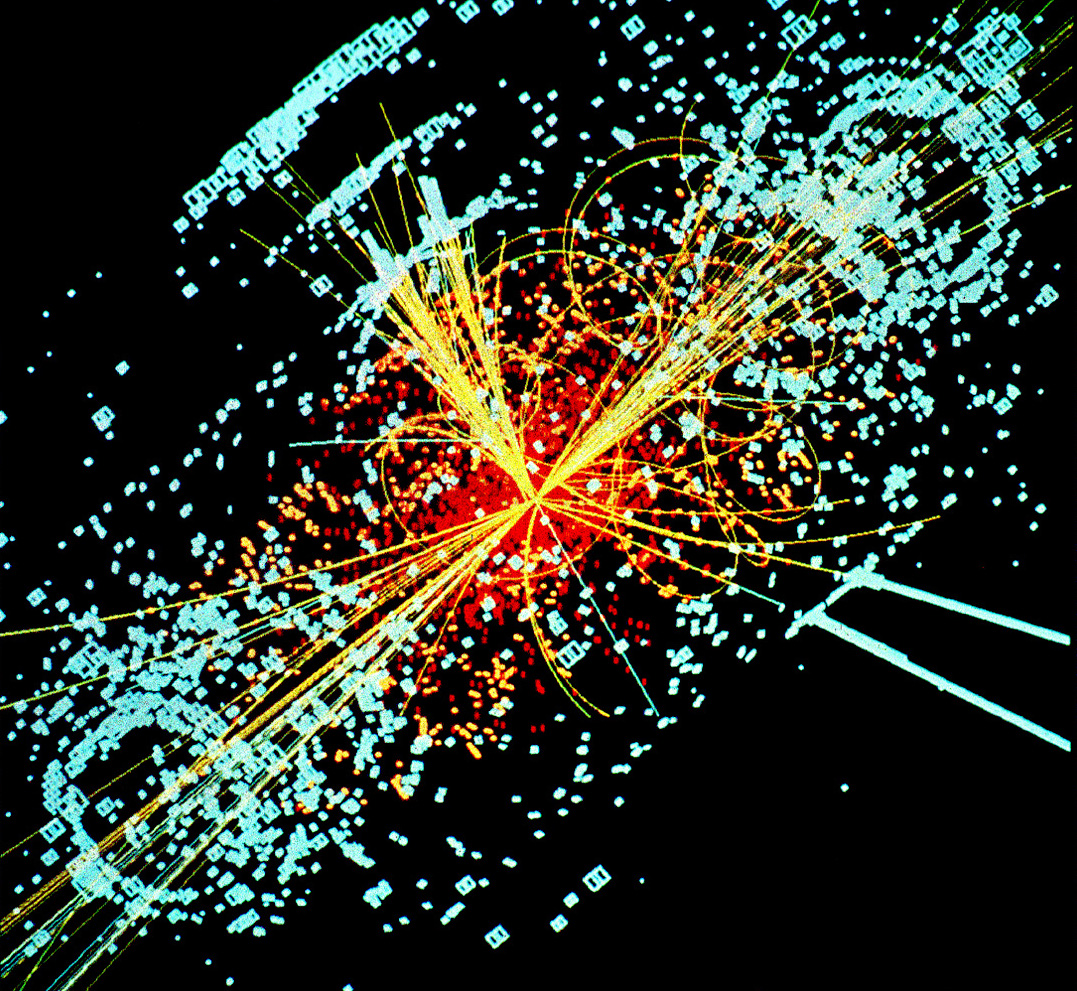
Confinement
A key phenomenon in Yang-Mills theory, coupled to some types of matter:

Particles carrying nonabelian electric charge are never observed. Only combinations with zero total charge can exist as isolated particles.
For example: confinement means we never see quarks by themselves, only bound together into neutral combinations.
Detecting confinement
One symptom of confinement: potential energy of a quark-antiquark pair grows linearly with the separation

How to formulate this directly in the language of QFT?
Not easily expressed using correlation functions of local operators: those involve measurements localized both in space and time, but our quark-antiquark are extended in time!
The Wilson loop
Ken Wilson, 1974: model a quark and antiquark with charges in representation $R$ as infinitely heavy external probes. Build a loop in spacetime; long sides represent the quark and antiquark, short sides included for technical convenience.
Measure fields along this loop:
$$ W_R = {\mathrm {Tr}_R}\,{\mathrm{Pexp}}\,\oint A_\mu d x^\mu $$
This is an example of a line defect.
For large $L$ and $T$, $\langle W_R \rangle$ obeys one of:
$\log \langle W_R \rangle \sim -LT$: confinement ("area law")
$\log \langle W_R \rangle \sim -(L+T)$: deconfinement ("perimeter law")
So does that explain confinement?
Not yet.
Having the Wilson loops $W_R$ available gives us a sharp criterion for what confinement means, and lets us test it, say, by lattice simulations.
But it's not easy to see from first principles why $\langle W_R \rangle$ would obey area law.
For that, we need another kind of loop...
The 't Hooft loop
Instead of measuring fields along the loop, we create a singularity for the fields as they approach the loop:
$$ F_{kj} = \frac{B}{4} \epsilon_{ijk} \frac{x^i}{\lvert{x}\rvert^3} $$The allowed $B \in {\mathfrak g}$ form a discrete set, depending on the group $G$ (analog of the set of representations of $G$.)
This represents insertion of heavy magnetically charged particles (nonabelian monopoles) instead of electric ones.

Dual confinement
In 1978 't Hooft pointed out a natural way the loop $\langle T_B \rangle$ could get area law: it happens if the theory is in Higgs phase (condensation of electrically charged field).

Now suppose that there is a dual description of the theory, such that $W$ in the original description is $T$ in the new description:
$$ W_R \leftrightarrow T_B $$In this case, confinement is the (dual) Higgs mechanism!
Montonen-Olive duality
In 1977 Claus Montonen and David Olive made a startling proposal: a dual description of Yang-Mills theory exists, and it is actually Yang-Mills theory again, in a new set of variables!
The two descriptions have different couplings:
$$g_{dual} = 1 / g$$so when one is weakly coupled, the other is strongly coupled.
It's a bold claim: says the limit of very large nonlinearity $(g \to \infty$) has another description in which it looks almost linear ($g_{dual} \to 0$).
Electromagnetic duality
In the case of Yang-Mills theory for $G = U(1)$, i.e. electromagnetism, Montonen-Olive duality is true (and easy)!
It is related to the fact that source-free Maxwell's equations
$$ \nabla \cdot \vec E = 0 \quad \nabla \times \vec E = - \partial_t \vec B $$ $$ \nabla \cdot \vec B = 0 \quad \nabla \times \vec B = \partial_t \vec E $$exhibit electromagnetic duality symmetry
$$ \vec E \to \vec B, \qquad \vec B \to - \vec E $$The full Montonen-Olive duality is like a nonlinear version of this. But can't be phrased directly as a symmetry of a system of equations.
${\mathcal N} = 4$ super Yang-Mills
It turns out Montonen-Olive duality is not true for ordinary Yang-Mills theory.
For a long time nobody seriously believed any version of the duality...


But in 1994, computations by Ashoke Sen, Cumrun Vafa and Edward Witten suggested it is true for a variant of Yang-Mills theory, ${\mathcal N} = 4$ super Yang-Mills.
This theory involves Yang-Mills field plus a bunch more fields, added in a specific way, so that the total theory has an extra symmetry called supersymmetry.
The dual group
Carefully matching Wilson and 't Hooft line defects shows that in general Montonen-Olive duality must relate different Yang-Mills theories:
$$ G \leftrightarrow \, ^L G $$where $^L G$ is the Goddard-Nuyts-Olive dual group.

 $$ \begin{array}{c|c}
G & ^L G \\ \hline
SU(N) & SU(N) / {\mathbb Z}_N \\
SO(2N+1) & Sp(N) \\
SO(2N) & SO(2N) \\
U(1) & U(1)
\end{array}
$$
$$ \begin{array}{c|c}
G & ^L G \\ \hline
SU(N) & SU(N) / {\mathbb Z}_N \\
SO(2N+1) & Sp(N) \\
SO(2N) & SO(2N) \\
U(1) & U(1)
\end{array}
$$
Defects and locality
We just said that there is a duality that relates Yang-Mills theories with groups
$$G = SU(N) \quad \text{ vs } \quad ^L G = SU(N) / {\mathbb Z}_N$$The difference between these two Yang-Mills theories is subtle!
They have the same correlation functions of local operators on ${\mathbb R}^4$. Nevertheless they are different theories.
This has sometimes caused puzzlement, since we are taught that one of the bedrock principles of QFT is that it is local. Shouldn't we be able to reconstruct the whole theory from its behavior on ${\mathbb R}^4$?
Incorporating defects into the definition of the theory provides a way out: the two theories are different because they have different line defects, even locally!
Another duality
An unexpected payoff from keeping careful track of these subtleties:
Michael Atiyah noticed that the duality
$$ G \leftrightarrow \, ^L G $$is the same one which appears in the Langlands program in number theory!


In 2006 Anton Kapustin and Edward Witten showed that this is not a coincidence: the geometric version of the Langlands program comes from Montonen-Olive duality. Careful attention to line defects is a key part of the story.

Line defects in general
Line defects have turned out to be a powerful probe of phases and dualities in quantum field theories, beyond ur-example of ${\mathcal N=4}$ super Yang-Mills:
-
In other super versions of Yang-Mills, Nathan Seiberg and Edward Witten in 1995 used electromagnetic duality to show that 't Hooft's picture of confinement via line defects is actually realized.
-
Two groups (Davide Gaiotto, Greg Moore and AN in 2010; Ofer Aharony, Nathan Seiberg and Yuji Tachikawa in 2013) used line defects to show that there are many other variants of Yang-Mills theory which had been overlooked before!


Onward and upward
So far we've discussed uses of local operators and line defects.
Next up: surface defects.
Solenoids
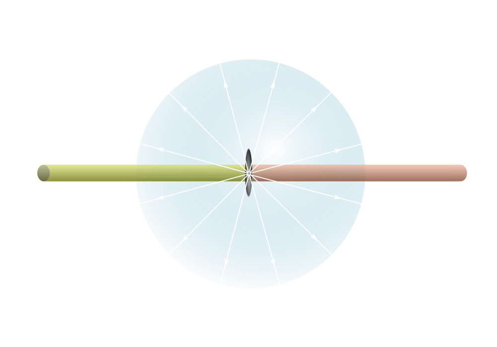
Back to electromagnetism.
Take a solenoid carrying an electric current. Then there is a magnetic flux threaded through the tube.

From long distance, solenoid looks like it's on a line in space; a surface in spacetime. So this is a surface defect.

Phases for a surface defect
Flux doesn't leak out of the solenoid, but it still affects dynamics of electrically charged particles outside: captured by Aharonov-Bohm phase
 $$ \Phi_e = \exp \left(i \int \!\!\! \int B_z\,dx\,dy\right) \in U(1) $$
We could also consider a surface carrying both electric and magnetic fluxes; then we would have two phases
$$ (\Phi_e, \Phi_m) \in U(1)^2 $$Thus the parameter-space of this surface defect is a torus.

Interfaces
Now suppose the solenoid has a break in it, where flux can escape; like a fractionally charged heavy particle.
This is an interface: line defect stuck on the surface defect.

Interfaces by varying surface defects
An interface can be built by continuously varying the parameters of a surface defect over a short distance scale.
i.e. we can get an interface from a path on the parameter-space of surface defects.

Line defects by varying surface defects
A crucial special case: we could consider the trivial surface defect, where
$$\Phi_e = \Phi_m = 1$$An interface between trivial surface defects just means a line defect!
So, line defects (e.g. Wilson, 't Hooft) can be built from closed loops on the parameter-space of surface defects.

Surface defects in Yang-Mills theory
How about surface defects in Yang-Mills theory?
For some supersymmetric variants there is a surprisingly pretty story, in which the torus gets replaced by another parameter-space.
e.g. in ${\mathcal N}=2$ super Yang-Mills with
$$G = SU(2) \times SU(2) \times SU(2)$$coupled to some specific matter fields, there are surface defects whose parameter space is a genus 2 surface.

(A really quantum phenomenon: can't see this by classical reasoning about Aharonov-Bohm phases!)
Surfaces and QFTs
It turns out that you can take any 2-dimensional parameter-space $C$ as starting point, and construct a corresponding four-dimensional QFT with ${\mathcal N = 2}$ supersymmetry (Witten, Gaiotto-Moore-AN, Gaiotto, 2009).
Very unlike the usual way of building a QFT by writing down fields and action. Most of these theories have no perturbation theory: need new tools.
The surprising point here: a priori, $C$ only knows about properties of surface defects in the theory. Yet somehow, $C$ (plus a little extra discrete data) seems to be enough to determine the whole $4$-dimensional theory!
The power of surface defects
The $4$-dimensional theory is controlled by the $2$-dimensional parameter-space $C$:
- line defects correspond to loops on $C$
- couplings determined by shape of $C$ (lengths of tubes)
- supersymmetric particle spectrum computed using string networks on $C$
- low-energy effective physics determined by certain contour integrals of multivalued functions over $C$
- dualities correspond to maps of $C$ to itself: huge generalization of Montonen-Olive!
- some correlation functions computable by a 2-dimensional QFT which lives on $C$!


Defects on defects
So far we've discussed local operators, line defects, surface defects, and interfaces (line defects on surface defects.)

One more easy example: local operators on line defects, e.g. a charged field gives an interface between different Wilson lines.

In general we can have defects of any dimension $d$, up to domain walls / boundary conditions.
Defects of dimension $d$ can have interfaces of dimension $d-1$, interfaces between interfaces of dimension $d-2$, $\dots$
Topological QFT
How to organize this zoo?
Consider a simplified model: the case of topological QFT. Very loosely this means a QFT where everything is invariant under homotopies (smooth deformations). In particular, distances are unimportant.
This class of QFT's has been intensively studied both by physicists and mathematicians, beginning with influential work of Witten in the late 1980's.
Two key examples:
- Chern-Simons theory in 3 dimensions: correlation functions of line defects are knot invariants.
- Donaldson-Witten theory in 4 dimensions: correlation functions of local operators and surface defects, on a compact Euclidean spacetime, compute 4-manifold invariants.
Extended topological QFT
Work of Ruth Lawrence and Dan Freed demonstrated by 1992-93 that a good framework for understanding locality in topological QFT is extended field theory, framed in the language of higher categories.
Later it was understood that these ideas can be interpreted very elegantly in terms of defects (e.g. as set out very clearly in a 2010 ICM address by Anton Kapustin):

Let's see how this works.
$0$-category of local operators
Local operators form a set, or $0$-category.

$1$-category of line defects
Line defects and interfaces form a richer structure: a set of objects (line defects) plus a set of morphisms between any two objects (interfaces).

Pushing the interfaces together along the line defect gives composition: combine two morphisms to make a third. (This is the moment where we use the topological nature of the QFT.) This operation is associative.

Altogether this says line defects form a $1$-category.
$1$-categories
$1$-categories are much beloved structures for (many) mathematicians: they can be found everywhere, e.g.
- the category whose objects are sets and morphisms are maps of sets,
- the category whose objects are vector spaces and morphisms are linear maps,
- the category whose objects are smooth spaces and morphisms are smooth maps,

- the category whose objects are representations of a group $G$ and morphisms are linear maps compatible with $G$ action,
- the category whose objects are points of some space $X$ and morphisms are homotopy classes of paths on $X$,
- $\cdots$
$2$-category of surface defects
Surface defects, interfaces, and interfaces between those form a yet richer structure: objects, morphisms, and morphisms-between-morphisms i.e. $2$-morphisms.

Topological property means there are several kinds of compositions of arrows (push interfaces together in various ways), obeying various associativity constraints, which look very complicated if you write them out.
Altogether this says: surface defects in a topological QFT form a $2$-category.
$n$-category of $n$-dimensional defects
In a similar way, $n$-dimensional defects in topological QFT form an $n$-category.
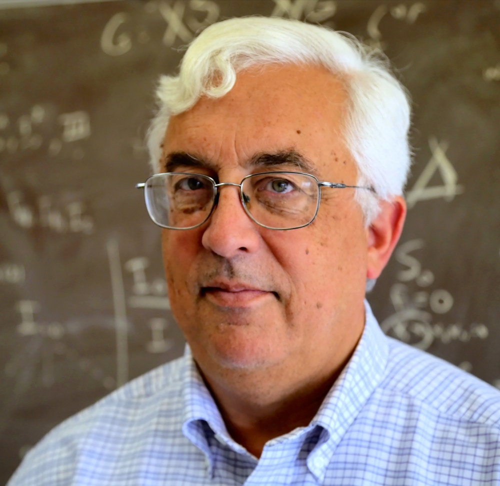
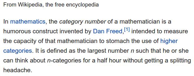
Historically these are less universally beloved objects:
The cobordism hypothesis
What are all these $n$-categories good for? How much information do they have about the topological QFT?
In 1995 John Baez and James Dolan proposed that the answer is all of it. Ignoring "technical details" their proposal is:


A topological QFT in $d$ dimensions is determined by its $(d-1)$-category of boundary conditions, and conversely, every $(d-1)$-category determines some topological QFT in $d$ dimensions!
This is now a theorem, proven by Michael Hopkins and Jacob Lurie (around 2010). But for some reason everyone still calls it the Cobordism Hypothesis.


Cutting up spacetimes
A loose interpretation of the Cobordism Hypothesis:
Suppose we want to compute a correlation function on some compact spacetime $X$. Locality suggests that we can chop $X$ into pieces so the interior of each piece has the topology of ${\mathbb R}^d$, evaluate the contribution from each piece, then glue them all together along their boundaries.

"Glue together" should mean something like "sum over all boundary conditions on the faces." The boundaries meet at corners, so also need to sum over interfaces at the corners, and so on at the deeper corners, $\dots$
Cobordism Hypothesis loosely says: this can really be done!
Almost done
Two closing remarks...
Extended TFT and condensed matter
Ideas from extended TFT have recently been put to serious use in the theory of topologically ordered phases in condensed-matter systems.
If you want to know about this: ask the real experts. We have a lot of them here!
A hopeful view
Two key ideas from this talk:
-
Thinking about the categories of defects has resolved thorny issues of what exactly locality means in topological field theory.
-
Defects and defects-on-defects are also very powerful in applications of non-topological field theory in high energy physics.
A hope, currently being actively pursued by many workers (including some at this workshop): maybe an upgraded version of these categorical ideas can help to finally define full-fledged, non-topological QFT.
That's it
Thank you!
That's it
Thank you!