Matrix Completion

I compiled some notes on low-rank matrix completion, with the goal of making the intuition behind the topic acessible to anyone proficient in linear algebra, but not familiar with basic convex optimization. There is no novel work here; I am presenting the work of Candès and Recht (2008), Candès and Tao (2009), and Recht (2010).

Problem Statement

In many applications, we wish to recover rank-$r$ $n$ by $n$ matrix $M$, of which we have only measured a subset of the entries. Let the indices of $m$ measured entries be $\Omega \subset \{1,…,n\} \times \{1,…,n\}$. If $m \ll n^2$, is it possible to recover this matrix exactly?

Of course, in general, it is not possible to do this: all of the $n^2$ measurements are needed. But if the rank $r$ is small, there is hope, as the number of degrees of freedom is $nr + r(n-r) \ll n^2$ (first choose $r$ linearly independent columns of size $n$ and then choose $r$ coefficients defining the linear combination that forms each of the remaining $(n-r)$ vectors). Since the actual dimensionality of this matrix is so much smaller than $n^2$, perhaps a similarly small number of elements, sampled randomly, will be sufficient for recovering it.

A very reasonable attempt at recovery might be to ask for the lowest rank matrix that agrees with our measurements. That is,

$\begin{align} \text{minimize } &\quad \text{ rank} (X) \tag{P0} \\ \text{such that } &\quad X_{ij} = M_{ij}\quad (i,j) \in \Omega. \end{align}$

However, this optimization problem is NP-hard to solve. The problem is that we are minimizing the the $\ell_0$ norm of the singular values (i.e. the rank). Candès and Recht (2008) had the insight to consider the convex relaxation of this problem, i.e. to minimize the $\ell_1$ norm of the singular values (called the nuclear norm, which we denote by $\| \cdot \|_*$ ).

$\begin{align} \text{minimize } &\quad \| X \|_* \tag{P1}\\ \text{such that } &\quad X_{ij} = M_{ij}\quad (i,j) \in \Omega. \end{align}$

In contrast to P0, the optimization problem P1 is convex and much easier to solve, even for large matrices! We can optimize this program, no problem, but will it give us the right thing? Specifically, we need to know if the true matrix $M$ is the unique solution to (P1).

In order to answer this question, we need some background in convex optimization.

Preliminaries

Matrix spaces and their norms

We will define an inner product of two matrices $A,B \in \mathbb R^{n_1 \times n_2}$ to be $\left\langle A, B \right\rangle = \text{tr}(A^T B) = \sum_{i,j} A_{ij}B_{ij}$. Denote the singular vector decomposition (SVD) of a matrix $M$ as $M=U\Sigma V^T$ and let $\sigma$ be the singular values, i.e. the diagonal of $\Sigma$. The Frobenius norm of $M$ is the sum of squares of the elements in $M$,

$\| M \|_F^2 = \left\langle M, M \right\rangle = \sum_{(i,j)} M_{ij}^2,$

and it is also the sum of the squares of the singular values. This can be seen simply as

$\| M \|_F^2 = \text{tr}(M^TM)= \text{tr}(V \Sigma U^T U \Sigma V^T) = \text{tr}(V \Sigma \Sigma V^T) = \sum_i \sigma_{i}^2 = \| \sigma \|_2,$

where the last equality used the fact that the trace is invariant under cyclic permutations, i.e. three matrices $A,B,C$, $\text{tr}(ABC) = \text{tr}(CAB)$.

Another useful norm is the operator norm, defined as

$\|M\|_{op} = \sup_{\|x\|_2 \leq 1} \| Mx \|_2 = \max_i \sigma_i = \| \sigma \|_\infty,$

i.e. the largest singular value of the matrix.

Finally, we have the nuclear norm,

$\| M \|_* = \sum_i |\sigma_{i}| = \| \sigma \|_1,$

which is simply the sum of the singular values (note that the absolute value sign is redundant; singular values are non-negative).

Importantly, note that the Frobenius, operator, and nuclear norms are the $\ell_2$, $\ell_\infty$, and $\ell_1$ norms of the singular values, respectively.

We can also introduce the orthogonal decomposition

$\mathbb R^{n_1 \times n_2} = T \otimes T^\perp,$

where $T$ is the space spanned by matrices of the form $u_k x^T$ and $yv_k^T$ for $1\leq k\leq r$ and any $x\in \mathbb R^{n_2}$ and $y \in \mathbb R^{n_1}$. The projection operator $\mathcal P_T: R^{n_1 \times n_2} \rightarrow T$ is defined by

$\mathcal P_T(X) = P_UX + XP_V - P_U X P_V,$

where $P_U$ and $P_V$ denote the orthogonal projection onto $U$ and $V$, respectively. Similarly, $\mathcal P_{T^\perp} = (\mathcal I - \mathcal P_T)(X)$, where $\mathcal I$ is the identity operator.

Finally, we use $P_\Omega$ to denote the sampling operator which sets all elements of a matrix to zero, except for the indices in $\Omega$.

Dual norms

Let $X$ be a vector space equipped with the norm $\|\cdot \|$ (for example, $\mathbb R^n$ with $\| \cdot \|_1$ ). Now, we can talk about the space $ X^* $ which consists of linear functionals on $X$, i.e. all $f : X \rightarrow \mathbb R$ such that $f$ is linear. This is called the dual space. If we want to define a norm $\| \cdot\|^*$ on this space of functionals, then it is natural to use the operator norm:

$\|f\|^* = \sup_{\| x\| \leq 1 } | f(x) |.$

That is, if you give $f$ any vector with norm less than 1, what is the largest number that can come out?

We will consider two concrete examples in finite dimensional spaces that will be useful to us below. First, it is helpful to realize that in an inner product space, linear functionals are simply inner products (this is called the Riesz Representation Theorem).

In an inner product space $(X,\left\langle \cdot , \cdot \right\rangle)$, for every linear functional $f : X \rightarrow \mathbb R$, there exists a unique $z \in X$ such that $f(x) = \left\langle x,z \right\rangle$.

Proof.

The Riesz Representation Theorem holds for any Hilbert space $X$, but since we will only consider finite dimensional vector spaces in these notes, we will only prove that special case (where it is trivial). Let $u_1,...,u_r$ be an orthonormal basis for the $r$ dimensional space $X$. Let $z = \sum_i f(u_i)u_i$, and note that $$ \begin{align*} \left\langle x, z \right\rangle &= \left\langle \sum_i a_i u_i, \sum_i f(u_iu_i\right\rangle\\ &= \sum_i a_if(u_i)\left\langle u_i, u_i\right\rangle\\ &= \sum_i a_if(u_i)\\ &= f\left(\sum_i a_iu_i\right)\\ &= f(x)\\ \end{align*} $$ $$\tag*{$\blacksquare$}$$

What is the dual space (and dual norm)? It is the vector space of all the linear functionals $f : \mathbb R^n \rightarrow \mathbb R $. Equipping $ \mathbb R^n $ with the natural inner product (i.e. the dot product), we can use the Riesz Representation Theorem from above, which states that any such linear functional can be represented by an element of $\mathbb R^n$. That is, for every $f$, there exists a $y$ such that $f(x) = \left\langle y ,x \right\rangle$.

The dual of $\| \cdot \|_1$ on $\mathbb R^n$ is $\| \cdot \|_\infty$ . That is,

$\|y\|_\infty = \sup_{\| x\|_1 \leq 1 } | \left\langle x,y \right\rangle |.$

This makes intuitive sense as well. Given $y$, how can you make $\left\langle x,y \right\rangle $ have a large absolute value, when you can only use $x$ with $\|x\|_1 \leq 1$ ? You need to put all the mass of $x$ onto the maximum element of $y$. The converse is true as well; the dual norm of the $\ell_\infty$ norm is the $\ell_1$ norm.

A second example is the space of matrices $\mathbb R^{n_1\times n_2}$, equipped with the inner product defined above. Analogously to the duality between $\ell_1$ and $\ell_\infty$, the dual of the operator norm is the nuclear norm.

We also have the Holder inequality for these dual norms,

$\left\langle A,B \right\rangle \leq \|A\|_1 \|B\|_\infty$

Lagrangian duality

Suppose we are interested in minimizing the following constrained optimization problem

$\begin{align*} \text{minimize } &\quad f(x,y)\\ \text{such that } & g(x,y) = c. \end{align*}$

A necessary condition for there to be a solution at $(x,y)$ is that there exists $\lambda$, such that

$\mathit L(x,y,\lambda) = \nabla_{x,y} f - \lambda \nabla_{x,y} g = 0.$

To borrow Wikipedia’s excellent explanation, consider the contour lines of $f$ and $g$. Of course, a solution must be on the contour line of $g$ corresponding to $g(x,y)=c$ for it to be reasible. So we can think about walking along this line, trying to find a minimum of $f$. A feasible minimum of $f$ will occur when the tangets of the contour lines of $f$ and $g$ are parallel. That is, where the contour line is $g=c$ is just “kisssing” (source) a contour line of $f$:

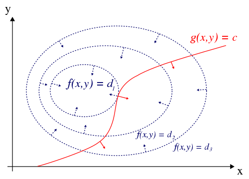
At such a point, there are no feasible points for which $f$ is any smaller…otherwise the tangents would not be parallel. If the tangents are parallel, then the gradients are also parallel. That is, there exists a $\lambda$ such that

$\nabla_{x,y} f = \lambda \nabla_{x,y} g,$

exactly the condition described above.

How about for P1? Here, we have $m$ constraints,

$g_k(X) = X_{i,j} - M_{i,j} = 0 ,$

by enumerating the elements of $\Omega$ as $k=1,…,m$ and letting $(i,j)$ be the $k$th index pair.

The equivalent condition to the 2D case, then, is the existence of $\lambda_1,…,\lambda_m$, such that

$\|X\|_* = \sum_{k=1}^m \lambda_k (X_{i,j} - M_{i,j}).$

Taking a gradient wrt $X$,

$\nabla g_k(X) = e_{i} e_{j}^T,$

i.e. the matrix of zeros with one in the $(i,j)$th entry. So, we have

$\nabla \|X\|_* - \sum_{k=1}^m \lambda_k e_{i,j} = \nabla \|X\|_* - P_\Omega \Lambda = 0,$

where $\Lambda \in \mathbb R^{n_1\times n_2}, $ and $P_\Omega$ sets all elements not in $\Omega$ to zero.

However, the nuclear norm is not differentiable, and hence we need to effectively replace the $\nabla$ with a sub-diffferential, in order to apply this approach.

Subgradients

Recall that a convex function lies above all its tangents. In fact, that is a definition of a convex function. If the function is differentiable, then its tangent at each point is well-defined. But if it’s not differentiable, there might be a set of tangents. This “set of tangents” is extremely useful for convex optimization.

A vector $g \in V$ is a subgradient of a convex function $f : V \rightarrow \mathbb R$ at $x_0$ if for all $z$,

$f(z) \geq f(x_0) + \left\langle g, z-x_0 \right\rangle$

In 1D, the picture (source) is especially clear:

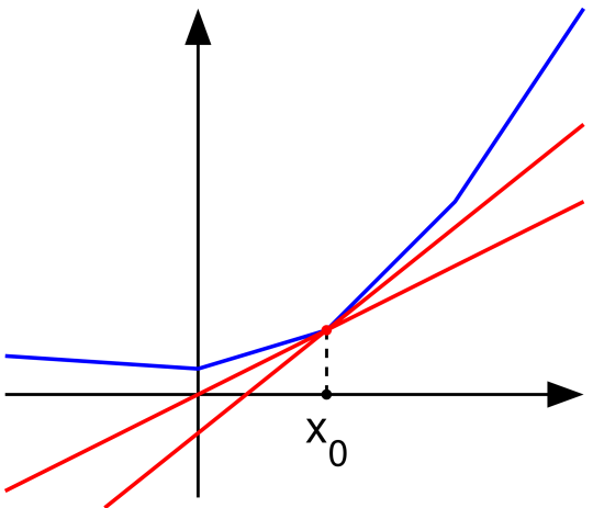
The red lines are subgradients of the function (blue) at a point $x_0$ where $f$ is not differentiable.

Recall that for a convex differentiable function, if $\nabla f(x_0) = 0$, then $x_0$ is a global minimum of $f$. It an exactly analogous with subgradients–except that now we ask if $0$ is in the set of subgradients. For convex $f$, if $0\in \partial f(x)$, then $x_0$ is global minimum because for any $h\in V$,

$\begin{align*} f(x_0+h) \geq f(x_0) + \left\langle 0, z \right\rangle = f(x_0) \end{align*}$

Clearly, the subgradient is useful for convex optimization! So let’s derive the subgradient for the nuclear norm at $X = U\Sigma V^T$. A formal derivation an be found in Watson (1992), below is some intuition for the direction we are interested in.

All matrices of the form $\{ UV^T + W : W \in \mathbb R^{n_1\times n_2}, \|W\|_{op} \leq 1, U^TW = 0, WV^T = 0 \}$ are subdifferentials of the trace norm at $X = U\Sigma V^T$.

Proof.

Let $$G = \{ UV^T + W : W \in \mathbb R^{n_1\times n_2}, \|W\|_{op} \leq 1, U^TW = 0, WV = 0 \}.$$ When function $f(x)$ is sup over set of functions $f_a$ indexed by compact set $A$ ( see e.g., here), $$ \text{conv} \left( \bigcup\limits_{\{s:f_s(x) = f(x)\} } \partial f_s \right)\subset \partial f(x).$$ That is, the convex hull of the subgradients of the functions $f_s$ that achieve the sup at that point are subgradients. $\| \cdot \|_*$ can be written in this form. Recalling that the nuclear norm is dual to the operator norm, $$\| X \|_* = \sup_{\|Y\| \leq 1} \text{tr}(Y^T X ),$$ we see that we only need to ask, which are the $Y$, with $\|Y\| \leq 1$, that maximize $\text{tr}(Y^TX)$? Decompose any $Y \in \mathbb R^{n_1 \times n_2}$ with $\| Y \| \leq 1$ as $$Y = \mathcal P_T(Y) + \mathcal P_{T^\perp}(Y),$$ where $T$ and $T^\perp$ are the subspaces of matrices defined above, but this time with respect to the SVD of $X$. This means that the value to maximize is $$\left\langle Y, X \right\rangle = \left\langle \mathcal P_T(Y), U\Sigma V^T \right\rangle + \left\langle \mathcal P_{T^\perp} (Y), U\Sigma V^T \right\rangle = \left\langle \mathcal P_T(Y), U\Sigma V^T \right\rangle,$$ which can be maximized by setting $\mathcal P_T(Y) = U V^T$. Furthermore, any $W$ with $\| W \| \leq 1$ can be added and the maximum will not change. Therefore, any matrix $Y$ such that,

$\mathcal P_T(Y) = U V^T$
$\|\mathcal P_{T^\perp}(Y) \|_{op} \leq 1$,

is a subderivative of the nuclear norm at $X = U\Sigma V^T$.

Therefore, if $Y$ is a matrix such that $\mathcal P_T(Y) = UV^T$ and $\| \mathcal P_{T^\perp} (W) \|_{op} \leq 1$ , then it is a subderivative of the nuclear norm at $M$.

What kind of matrices can be recovered?

It is not enough that the matrix simply be low rank. Consider the matrix $M = e_i e_j^*$, where $e_j$ is the $j$th standard basis vector, i.e. the vector of zeros where the $j$th element is 1, like

$\begin{bmatrix} 0 & 0 & 0 & 1 \\ 0 & 0 & 0 & 0 \\ 0 & 0 & 0 & 0 \end{bmatrix}$

No matter how you sample this rank-1 matrix, you need to have every value to recover it exactly.

Or consider the classical example of collaborative filtering, i.e. the “Netflix Problem.” Suppose Netflix keeps track of of every user’s ratings in a matrix form, where the rows correspond to movies, the columns correspond to users, and the element is the numeric rating (e.g. from 1-5) assigned to the movie by a given user. We call all the movies that the user has not seen “missing,” because we don’t know how much the user will like it. The matrix completion problem in this context is to estimate the scores the user would assign to each of the movies, if he/she saw them all.

It is easy to see that this matrix might be “approximately” low-rank, because there will be lots of correlation between the rows/columns. For example, say there were $m$ movies and $n$ users, so the $m\times n$ matrix was actually rank r, then its SVD can be written as

$M = \sum_{i=1}^r u_iv_i^T \sigma_i.$

One might imagine that each $u_i$ could correspond to a movie genre (e.g. action, adventure, romance, etc), and then $v_i$ determines how much each user “likes” that genre. Indeed, $u_i v_i^T\sigma_i$ is an $m \times n$ matrix that contains the contribution of that given genre to all the elements. Suppose, however, that $v_2 = e_1$, i.e. it is a vector of zeros with 1 in the first element. Such a matrix cannot be recovered, because all the information about $u_2$ is in the first column, and so we need to always sample every value in the first column to exactly recover this matrix.

In both these examples, the problem is that one of the singular vectors is a standard basis vector. A necessary condition for matrix completion is that none of the (left or right) singular vectors of the matrix are too correlated with the standard basis. This is quantified in a measure of “coherence” for a subspace, which measured how “spread out” the basis vectors are. Candès and Recht define the coherence of an $r$-dimensional subspace $U$ of $\mathbb R^n$ as

$\mu(U) = \frac{n}{r} \max_{1\leq i\leq n} \| P_U e_i \|^2,$

where $P_U$ is the orthogonal projection onto $U$. This can be thought of as a mesure of “how well can the subspace represent $e_i$.” That is, how “ordered” are they, or “concentrated,” with respect to the standard basis. Using coherence, we can now state the main theorem.

Some intuition

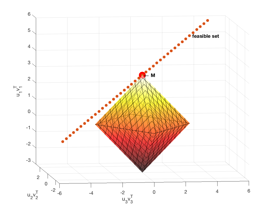
Before we state the main theorem, let’s get some intuition by letting $M$ be the rank-1, 3 by 3 matrix of ones. By computing the SVD of $M = \sum_{i=1}^3 \sigma_i u_i v_i^T$ where $\sigma_2$ and $\sigma_3$ are zero, we can visualize the subspace defined by linear combinations of the basis vectors $u_1 v_1^T$, $u_2 v_2^T$, $u_3 v_3^T$. The latter two are in $T^\perp$, whereas the first is in $T$. Of course, the space of all matrices 3 by 3 matrices is 9 dimensional, but visualizing these three can give some intuition.

Now, suppose we sample $M$ at all entries except for the upper right corner. By varying that entry, we can see the subspace (a line) of matrices that obey the constraint in P1 (i.e. the feasible set). P1 successfully recovers the true matrix $M$ when every other matrix on this line has a larger nuclear norm. We can visualize this scenario in the 3-dimensional space defined above.

Demo 3 by 3

% Let the true matrix be a rank-1 3 by 3 matrix of 1s. Suppose we sample
% all but its upper right corner.
M = ones(3);
[U S V] = svd(M);

[l1 l2  l3] = get_lambda3(M, U,V) % Note that this is just diag(S) here

figure(2);clf
scatter3(l3,l2,l1,200, 'red','filled');
txt1 = ' \leftarrow M'; t=text(l3,l2,l1,txt1);t.FontWeight = 'bold';

hold on

% Plot the projection of all feasible matrices into this 3 dimensional
% subspace. A feasible matrix is one where all values except the upper
% right corner are 1. 
feasibles = zeros(10,2);
replacements = -10:0.5:10
for ii=1:length(replacements)
    A2 = M;
    A2(2,2) = replacements(ii);
    [l1 l2 l3] = get_lambda3(A2, U,V);
    feasibles(ii,1) = l1;
    feasibles(ii,2) = l2;
    feasibles(ii,3) = l3;

end

global M_norm;
M_norm =sum(diag(S));

scatter3(feasibles(:,3),feasibles(:,2), feasibles(:,1),'filled')
txt1 = '  P_\Omega (X) = P_\Omega(M)';
t  =text(feasibles(end-5,3),feasibles(end-5,2), feasibles(end-5,1),txt1)
t.FontWeight = 'bold'

% Plot the L1 ball in this subspace (there might be a much cleaner way to
% do this...)
zfun = @(x,y) (abs(x) + abs(y) <M_norm ).*(M_norm - abs(x) - abs(y)) + (abs(x) + abs(y) >=M_norm ).*0
xfun = @(x,y) (abs(x) + abs(y) <M_norm ).*x + (abs(x) + abs(y) >=M_norm ).*M_norm.*x./(abs(x)+abs(y) + 0.001);
yfun = @(x,y) (abs(x) + abs(y) <M_norm ).*y +  (abs(x) + abs(y) >=M_norm ).*M_norm.*y./(abs(x)+abs(y) + 0.001);
hSurface = fsurf( xfun,yfun, zfun,[-M_norm M_norm -M_norm M_norm] )
set(hSurface, 'FaceAlpha',0.5, 'MeshDensity', 20)
hold on;
zfun = @(x,y) (abs(x) + abs(y) <M_norm ).*(-M_norm + abs(x) + abs(y)) + (abs(x) + abs(y) >=M_norm ).*0
hSurface = fsurf( xfun,yfun,zfun,[-M_norm M_norm -M_norm M_norm] )
set(hSurface, ...
  'FaceAlpha',0.5, ...
   'MeshDensity', 20)
colormap hot
zlabel('u_1v_1^T')
ylabel('u_2v_2^T')
xlabel('u_3v_3^T')



% A function that gives the projection of a 3 by 3 matrix onto the subspace
% defined by the following three basis "vectors": U(:,i) * V(:,i)' for i=1,..,3 

function [ l1,l2, l3 ] = get_lambda3( A, U,V )
u1 = U(:,1); u2 = U(:,2); u3 = U(:,3);
v1 = V(:,1); v2 = V(:,2); v3 = V(:,3);

l1 = u1'*A*v1;
l2 = u2'*A*v2;
l3 = u3'*A*v3;
end

Of course, we need to be careful about reading too much into this figure, because it is only 3 of the 9 dimensions. That being said, it still gives a nice intuition. For example, what if

$M = \begin{bmatrix} 1 & 5 & 2 \\ 1 & 5 & 2 \\ 0 & 0 & 0 \\ \end{bmatrix}$

Note that this is still a rank-1 matrix, but it is more “coherent.” Here is the same visualization:

Demo 3 by 3

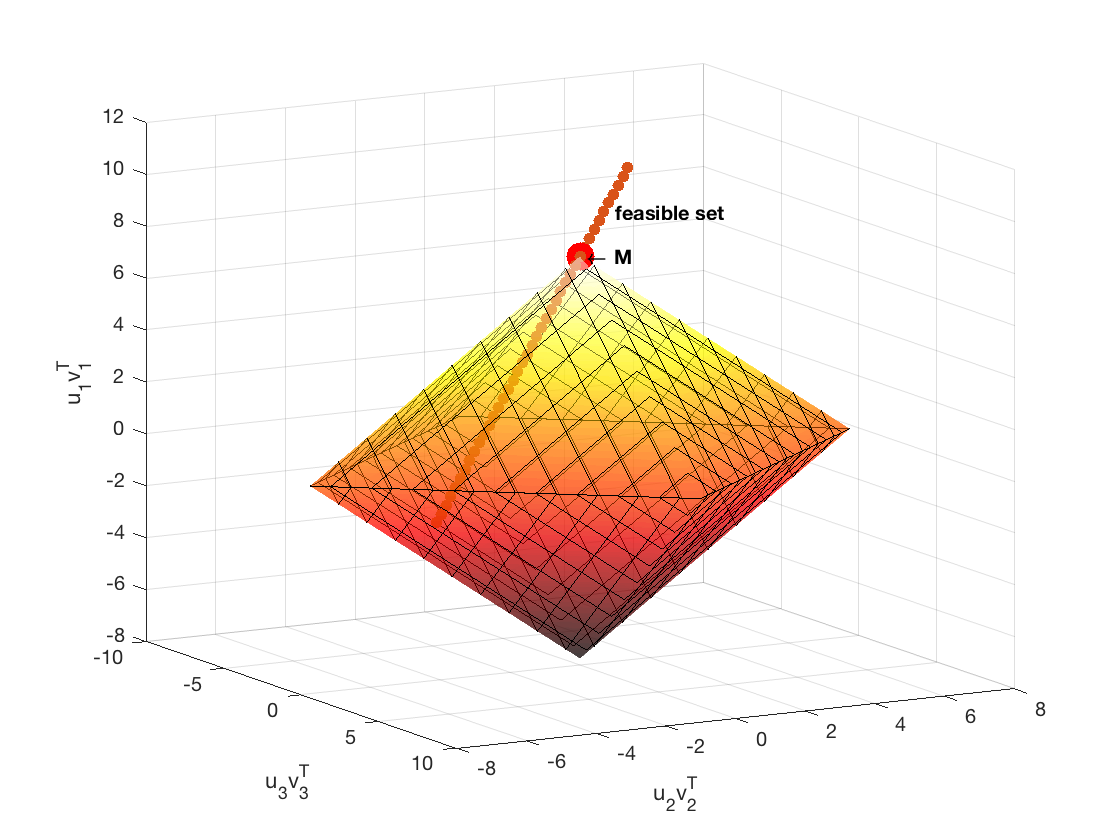
Note how there are feasible solutions with smaller $\ell_1$ norm of the coefficients in this subspace than $M$. This suggests that the matrix is not recoverable. This visualization also suggests how the subgradient works. Recall that a subgradient $Y$ has to have a coefficient of 1 on the $u_1v_1^T$ axis, and then if $W= \mathcal P_{T^\perp(M)},$ then $\|W\|_{op} \leq 1$ . This means that the angle between the $u_1v_1^T$ axis and $Y$ must be less than or equal to 45 degrees. So, if such a subgradient is in the range of the sampling operator, it means that the feasible set will only intersect with the $\ell_1$ ball at $M$.

Main Theorem

Before we state the main theorem, we need two assumptions about the matrix $M = \sum_{k=1}^r \sigma_k u_k v_k^*$, where column and row spaces are $U$ and $V$.

A0: Coherence of column and row spaces is bounded, i.e. $\max( \mu(U), \mu(V) ) \leq \mu_0$ for some positive $\mu_0.$

A1: The matrix $\sum_{k=1}^r u_kv_k^*$ has maximum entry bounded by $\mu_1 \sqrt{r/(n_1n_2)}$ in absolute value for some positive $\mu_1$

Note that A1 always holds with $\mu_1 = \sqrt{r} \mu_0$ because of Cauchy Schwarz, so won’t worry about it for small $r$.

Now, we can state a theorem of Candès and Recht (2008):

Let $M$ be $n_1 \times n_2$ matrix of rank $r$ obeying A0 and A1, and let $n= max(n_1,n_2)$. Suppose $m$ entries of $M$ are observed at locations sampled uniformly. Then there exist $C,c$ such that if $$m \geq C \max( \mu_1^2, \mu_0^{1/2}\mu_1, \mu_n^{1/4} ) nr(\beta \log n )$$ for some $\beta >2$, then the minimizer to P1 is unique and equal to $M$ with probability at least $1-cn^{-\beta}$. For $r \leq \mu_0^{-1} n^{1/5}$ this estimate can be improved to $$m \geq C \mu_0 n^{6/5} r ( \beta \log n)$$ with same probability of success.

Notably, Candès and Tao (2009) then further improved the number of sampled elements to be $m \sim nr\log^6 n$ which they showed was “nearly optimal.”

The proof of this theorem, and the improved bound by Candès and Tao, requires some heavy machinery beyond the scope of these notes. We will show, however, the general architecture of the proof, which is ubiquitous in this area of research. It comes from this lemma:

Consider $X_0 = \sum_{k=1}^r \sigma_k u_kv_k^*$ which is feasible for P1. Suppose the following conditions hold:

There exists dual point $\lambda$ such that $Y = P_\Omega \lambda$ which obeys $$P_T(Y) = \sum_{k=1}^r u_k v_k^*,\quad \|P_{T^\perp}(Y)\| < 1.$$
The sampling operator $P_\Omega$ restricted to elements in $T$ is injective.

Then $X_0$ is the unique minimizer.

Proof.

Consider $X_0 + H$, with $P_\Omega(H) = 0$. That is, any other matrix that is feasible for P1. To show that $X_0$ is the unique minimizer, we need to show that $$\|X_0 + H \| > \| X_0 \|.$$ For any $W_0 \in T$ with $\|W_0\|_{op} \leq 1$, $\sum_{i=1}^r \sigma_i u_i v_i^* + W_0$ is subgradient, so $$\|X_0 + H \|_{op} \geq \|X_0\|_{op} + \left\langle \sum_i \sigma_i u_i v_i^* + W_0, H \right\rangle$$ Letting $W=P_{T^\perp} (Y)$, by assumption, we have $\sum_i \sigma_i u_i v_i^* = P_\Omega\lambda - W$, so $$ \begin{align*} \|X_0 + H \|_{op} &\geq \|X_0\|_{op} + \left\langle P_\Omega \lambda + W_0 - W, H \right\rangle\\ &\geq \|X_0\|_{op} + \left\langle W_0 - W, H \right\rangle\\ \end{align*} $$
Now, just need to show that $\left\langle W_0 - W, H \right\rangle > 0.$ Because $W_0,W\in T^\perp$, $$\left\langle W_0 - W, H \right\rangle = \left\langle P_{T^\perp} (W_0 -W), H \right\rangle = \left\langle W_0 - W, P_{T^\perp} (H) \right\rangle$$ We set $W_0 = P_{T^\perp}(Z)$, where $\|Z\|_{op} \leq 1$ and $\left\langle Z, P_{T^\perp}(H) \right\rangle = \| P_{T^\perp(H)} \|_*$. Such a $Z$ exists because $\|\cdot \|_*$ and $\|\cdot\|_{op}$ are dual norms. $$ \begin{align*} \left\langle W_0 - W, H \right\rangle &= \left\langle W_0, P_{T^\perp} (H) \right\rangle - \left\langle W, P_{T^\perp}( H) \right\rangle\\ &\geq \|P_{T^\perp}(H)\|_* - \|W\|_{op} \| P_{T^\perp(H)} \|_*\\ &= (1 - \|W\|) \| P_{T^\perp(H)} \|_* \end{align*} $$ Which is strictly positive, unless $\| P_{T^\perp(H)} \|_* = 0$. But if it is zero, then $H \in T$ and $P_\Omega(H) = 0$, so by injectivity of $P_\Omega$ on $T$, $H=0$. Therefore, $\|X_0 + H \|_* > \|X\|_*$

That is, if we construct a dual certificate that is a subgradient of the nuclear norm at $M$, and we show that the sampling operator on $T$ is injective, we are done! Candès and Recht (2008), Candès and Tao (2009), and Recht (2010) all differ primarily in how they accomplish these tasks. Here we highlight the particularly simple and elegant approach of Recht (2010) that uses matrix concentration inequalities.

Simplification by sampling with replacement

Note that theorem is about uniform sampling of the matrix entries. However, in their proofs, Candès and Recht (2008) and Candès and Tao (2009) both use binomial sampling, then bound error of this approximation. Recht (2010) dramatically simplifies proof by using sampling with replacement and using matrix concentration inequalities.

Let $\Omega = { (a_{k}, b_k) }_{k=1}^m $ be collection of indices sampled uniformly with replacement. Define

$\mathit R_\Omega(Z) = \sum_{k=1}^{|\Omega|} \left\langle e_{a_k} e_{b_k}^*, Z \right\rangle e_{a_k} e_{b_k}^*.$

Note that this is not a projection operator if there are duplicates, but can easily bound the number of duplicates using a standard Chernoff bound.

Recht (2010) then uses this framework to construct an “approximate dual certificate,” and also show that the sampling operator $\mathit R_\Omega$ is injective on $T$. Here, we show only the latter, as it is a particularly elegant application of matrix inequalities.

To show that the sampling operator is injective, Recht (2010) shows that it is an approximate isometry:

Suppose $\Omega$ is set of $m$ entries sampled independently and uniformly with replacement. Then for all $\beta > 1$, $$\frac{n_1n_2}{m} \left\| P_T \mathit R_\Omega P_T - \frac{m}{n_1n_2} P_T \right\| \leq \sqrt { \frac{16 \mu_0 r(n_1 + n_2) \beta \log(n_2)}{3m}} = a$$ with probability at least $1-wn^{2-2\beta}$ provided that $m > \frac{16}{3} \mu_0 r(n_1+n_2) \beta \log(n_2)$.

Note that this is stronger than injectivity! For $X\in T$,

$\left\|P_T \mathit R_\Omega X - \frac{m}{n_1n_2}X\right\| < a \frac{m}{n_1n_2} \| X \|$

So, $\mathit R_\Omega$ cannot vanish, because otherwise

$\begin{align*} \frac{m}{n_1n_2} \|X\| &< a \frac{m}{n_1n_2} \| X \|\\ 1 &< a \end{align*}$

but $m$ is chosen to be large enough that $a <1 $.

To prove this theorem, Recht notes that

$\mathbb E P_T \mathit R_\Omega P_T = P_T \mathbb E \mathit R_\Omega P_T = \frac{m}{n_1n_2} P_T$

So, we are simply bounding the deviation of $ P_T \mathit R_\Omega P_T $ from its mean:

$\frac{n_1n_2}{m} \left\| P_T \mathit R_\Omega P_T - \frac{m}{n_1n_2} P_T \right\|,$

which is exactly where matrix concentration inequalities come in! Recht simply bounds the first and second moments, then applies Matrix Bernstein to obtain the above theorem. In Joel Tropp’s (absolutely excellent) review of matrix concentration inequalities, and he notes that this application is one of the first to popularize matrix concentation inequalities in machine learning and mathematical statistics.

Hopefully these notes were helpful; please feel free to contact me with any corrections, suggestions, or comments.

References

Candès, Emmanuel J., and Benjamin Recht. “Exact matrix completion via convex optimization.” Foundations of Computational mathematics 9.6 (2009): 717.
Candès, Emmanuel J., and Terence Tao. “The power of convex relaxation: Near-optimal matrix completion.” IEEE Transactions on Information Theory 56.5 (2010): 2053-2080.
Recht, Benjamin. “A simpler approach to matrix completion.” Journal of Machine Learning Research 12.Dec (2011): 3413-3430.